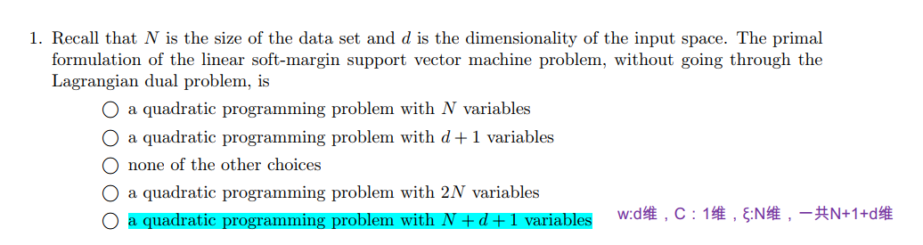
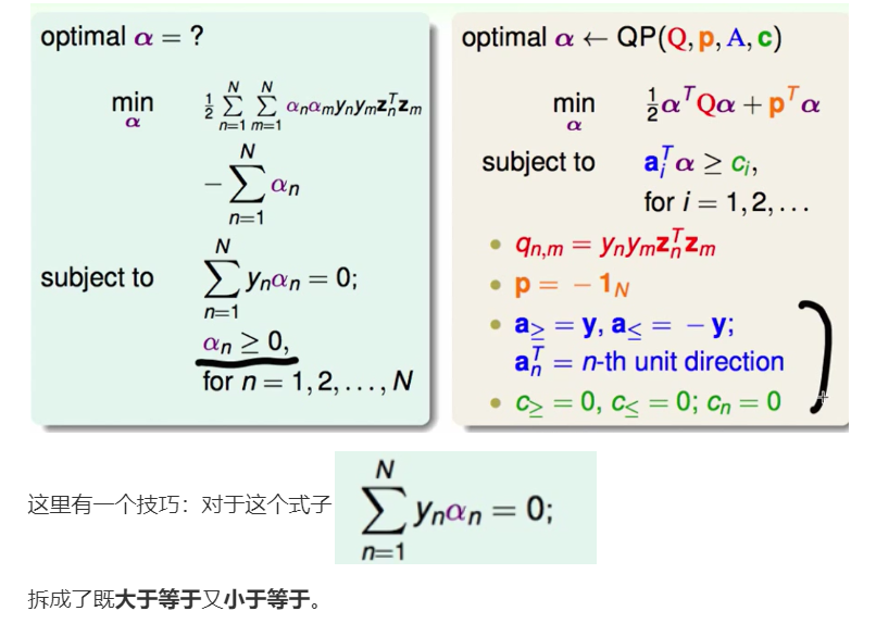
QUIZ 1: Q1
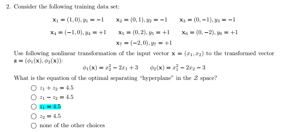
Q2
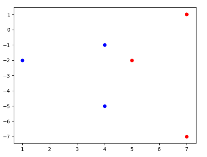
1
2
3
4
5
6
7
8
9
10
11
12
13
14
15
16
17
18
19
20
21
22
from cvxopt import solvers, matriximport numpy as npimport matplotlib.pyplot as pltdef z1 (x1,x2) :return x2**2 - 2 *x1 + 3 def z2 (x1,x2) :return x1**2 - 2 *x2 - 3 if __name__ == '__main__' :1 , 0 ], [0 , 1 ], [0 , -1 ], [-1 , 0 ], [0 , 2 ], [0 , -2 ], [-2 , 0 ]])-1 , -1 , -1 , 1 , 1 , 1 , 1 ]for vec in x:0 ], vec[1 ]), z2(vec[0 ], vec[1 ])])for i in range(len(y)):if y[i] == -1 :0 ], z[i][1 ], color='blue' )else :0 ], z[i][1 ], color='red' )
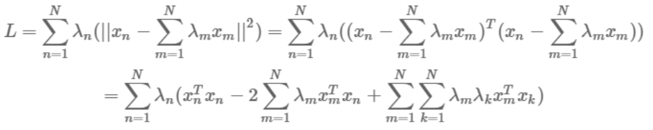
不难看出是在$z_1=4.5$处为分界面
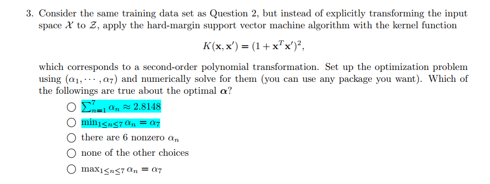
Q3
1
2
3
4
5
6
7
8
9
10
11
12
13
14
15
16
17
18
19
20
21
22
23
24
25
26
27
28
29
30
31
32
from cvxopt import solvers, matriximport numpy as npimport matplotlib.pyplot as pltdef kernel (x1, x2) :return (1 + np.dot(x1.T, x2))**2 if __name__ == '__main__' :1 , 0 ], [0 , 1 ], [0 , -1 ], [-1 , 0 ], [0 , 2 ], [0 , -2 ], [-2 , 0 ]])-1 , -1 , -1 , 1 , 1 , 1 , 1 ])7 , 7 ))for i in range(7 ):for j in range(7 ):7 )9 , 7 ))0 ] = y1 ] = -yfor i in range(2 ,9 ):-2 ] = -1 9 )'max alpha:' , np.max(alphas['x' ]))'alpha sum:' , np.sum(alphas['x' ]))'min alpha:' , np.min(alphas['x' ]))'alphas:' , alphas['x' ])
这里要注意下:cvxopt做二次规划和林轩田老师ppt上的
符号方向是相反的。
运行结果:
max alpha: 0.8888888987735439 alpha sum: 2.814814850082614 min alpha: 6.390795094251015e-10 alphas: [ 6.69e-09 ] [ 7.04e-01 ] [ 7.04e-01 ] [ 8.89e-01 ] [ 2.59e-01 ] [ 2.59e-01 ] [ 6.39e-10 ]
故1,2是正确的。
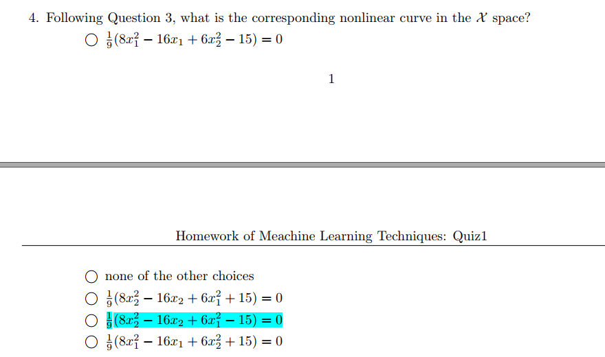
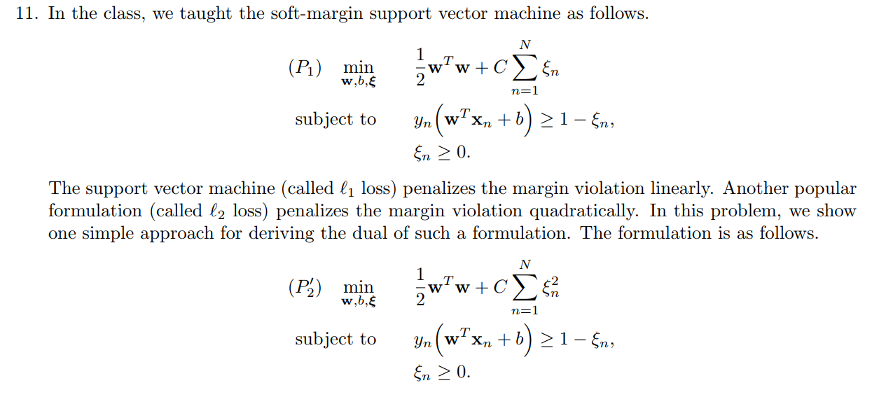
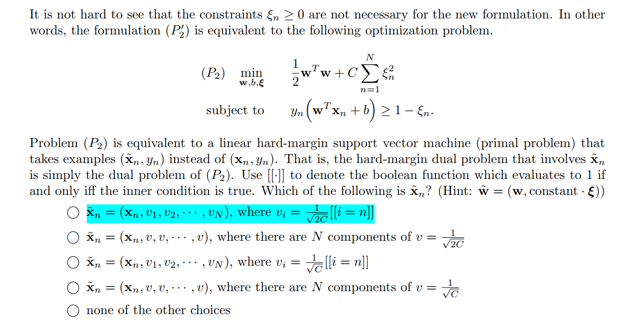
Q4
我们已知道$\alpha$,去求b即可,然后带回$g_{SVM}$.
1 2 3 4 5 6 7 8 9 10 11 12 13 14 15 16 17 18 19 20 21 22 23 24 25 26 27 28 29 30 31 32 33 34 35 36 37 38 39 40 41 42 43 from cvxopt import solvers, matriximport numpy as npimport matplotlib.pyplot as pltreturn (1 + np.dot(x1.T, x2))**2 if __name__ == '__main__' :array ([[1 , 0 ], [0 , 1 ], [0 , -1 ], [-1 , 0 ], [0 , 2 ], [0 , -2 ], [-2 , 0 ]])array ([-1 , -1 , -1 , 1 , 1 , 1 , 1 ])7 , 7 ))for i in range(7 ):for j in range(7 ):7 )9 , 7 ))0 ] = y1 ] = -yfor i in range(2 ,9 ):-2 ] = -1 9 )'x' ]return np.array ([x[0 ] * x[0 ], x[1 ] * x[1 ], 2 * x[0 ] * x[1 ], 2 * x[0 ], 2 * x[1 ], 1 ])6 )for i in range(7 ):1 ]for i in range(7 ):1 ])'x1*x1:' , w[0 ], 'x2*x2:' , w[1 ], 'x1*x2:' , w[2 ], 'x1:' , w[3 ], 'x2:' , w[4 ], '1:' , w[5 ])'b:' , b)
运行结果:
x1*x1: 0.8888888946403547 x2*x2: 0.666666683766254 x1*x2: 0.0 x1: -1.7777778134824205 x2: -3.3306690738754696e-15 1 : -1.586721330977244e-10 -1.6666666836075785
即第三个。
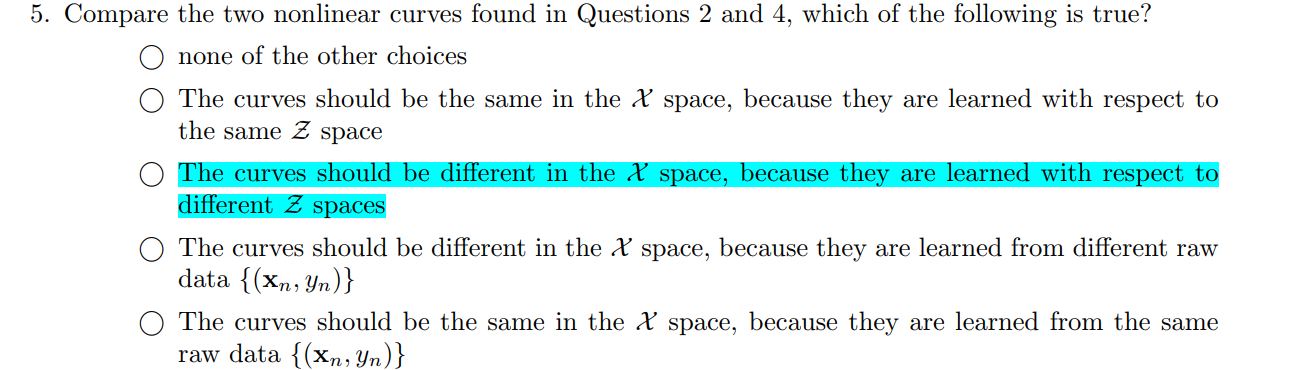
Q5
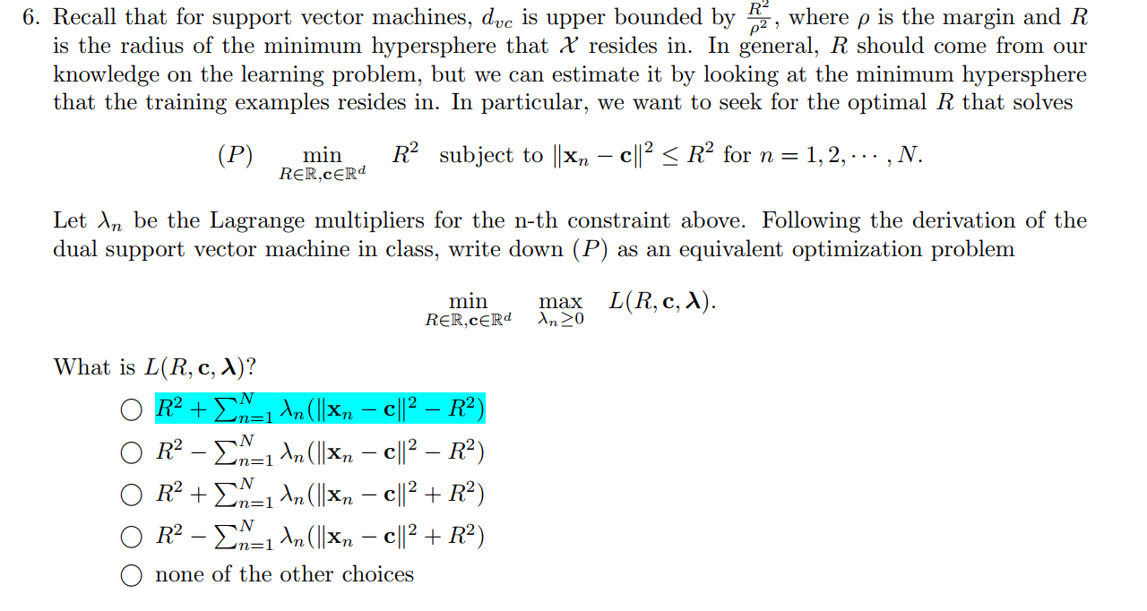
Q6
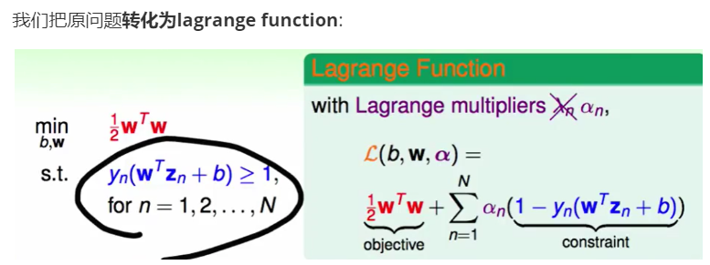
根据上面的ppt用lagrange multiplier转化为lagrange function即可:
要注意的是 ppt里给的是$\ge$, 而题目里是$\le$, 两边同加上负号,让符号方向就会转回来即可。
答案是第一个。
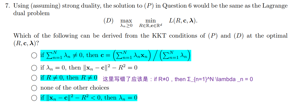
Q7
我们仿写KKT条件:
$\frac{\partial L(R,c,\lambda)}{\partial R}= R(1-\Sigma_{n=1}^N \lambda_n)=0$
$\frac{\partial L(R,c,\lambda)}{\partial ci}=0 \to c_i\Sigma {n=1}^N\lambdan =\Sigma {n=1}^N\lambda_nx_n^{(i)} $
这样就推出了第1,3个是正确的。
然后为来看第五个,就是KKT条件中所提到的:
我们仿写就是:$\lambda_n(||x_n-c||^2-R^2) = 0$
那么第5个也正确。
所以答案是1,3,5。
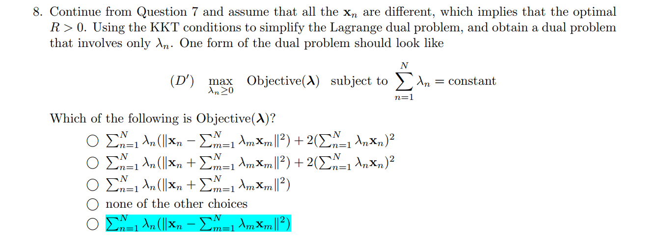
Q8
解析:
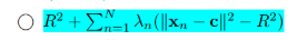
题目提到$R>0$,由Q7可知:$R(1-\Sigma{n=1}^N \lambda_n)=0$,故$1-\Sigma {n=1}^N \lambda_n=0$
原始的Lagrange Function在Q6中提到了:
我们把$1-\Sigma_{n=1}^N \lambda_n=0$带入:
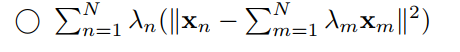
$\ \ \ R^2 + \Sigma{n=1}^N\lambda_n(||x_n-c||^2-R^2)\ = R^2 + \Sigma {n=1}^N\lambdan||x_n-c||^2-\Sigma {n=1}^N\lambdanR^2 \=\Sigma {n=1}^N\lambda_n||x_n-c||^2$
我们又由Q7中的式子:
$\frac{\partial L(R,c,\lambda)}{\partial ci}=0 \to c_i\Sigma {n=1}^N\lambdan =\Sigma {n=1}^N\lambda_nx_n^{(i)} $
又因为$1-\Sigma_{n=1}^N \lambda_n=0$,得到:
$ci\Sigma {n=1}^N\lambdan =\Sigma {n=1}^N\lambdanx_n^{(i)} \\to c_i = \Sigma {n=1}^N\lambda_nx_n^{(i)}$
带入$\Sigma_{n=1}^N\lambda_n||x_n-c||^2$得到第5个为正确答案:
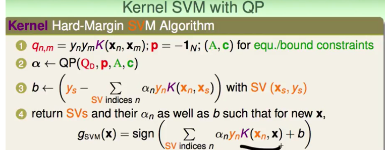
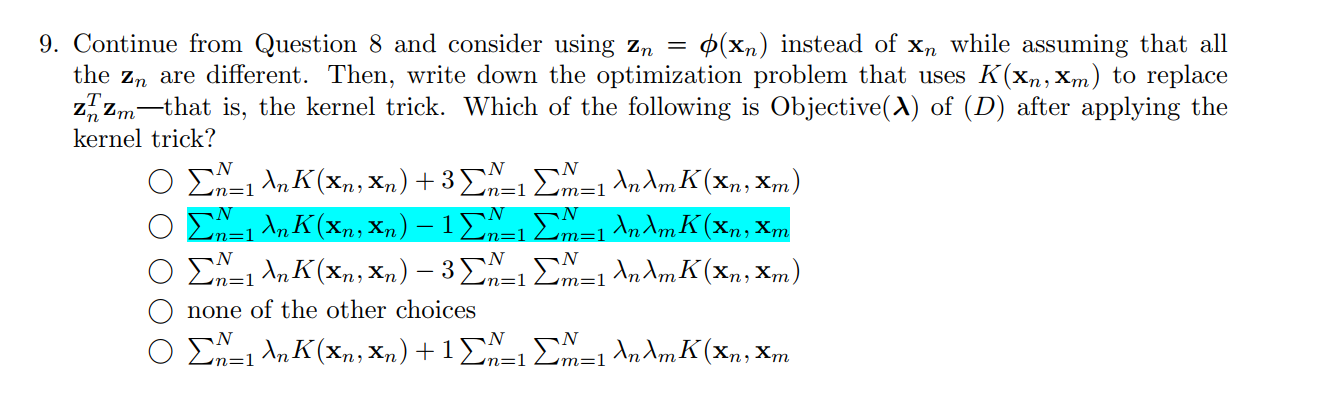
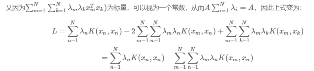
Q9
解析:
从Q8的结果加上kernel技巧就好:
Q10
解析:
选择$\lambda\ne 0 $的SV。
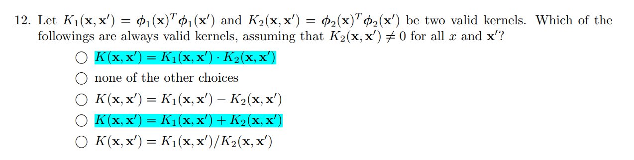
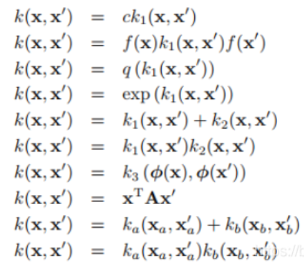
Q11
Q12
解析:
下面这些都可以:
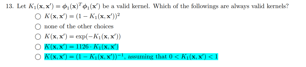
Q13
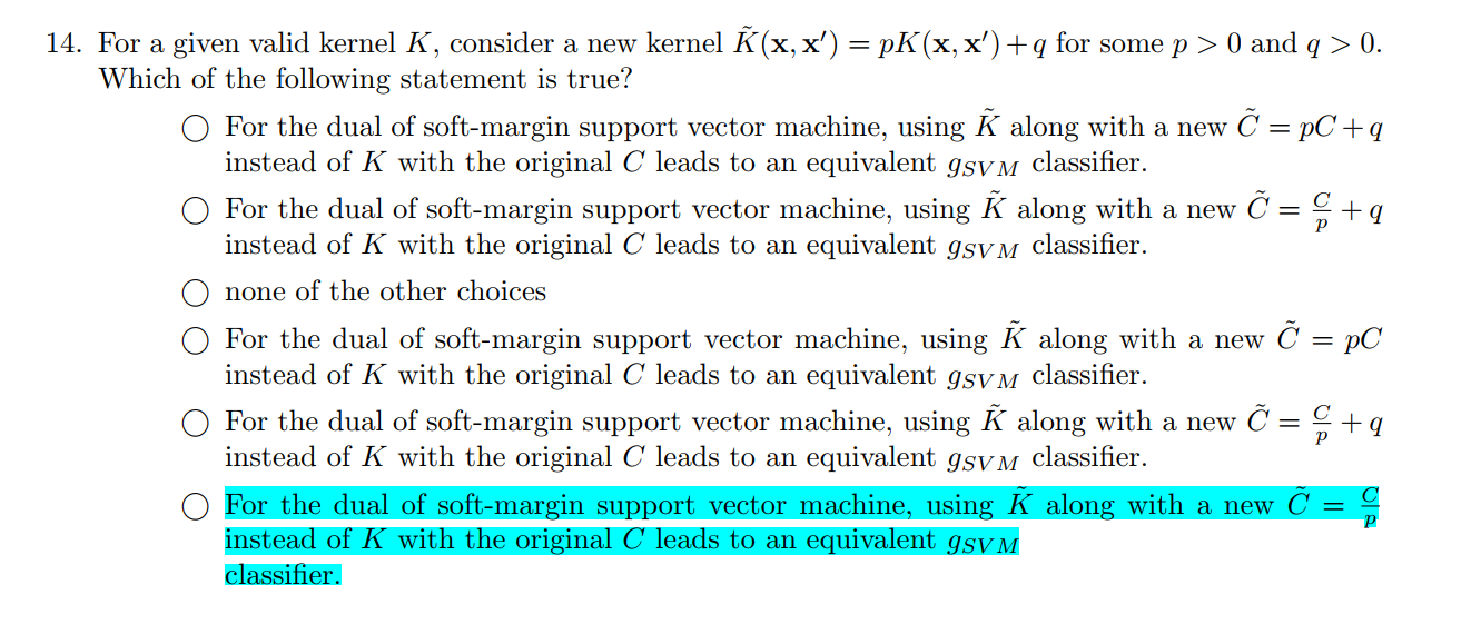
Q14
$K(x,x’)=z^Tz $,这里把$K(x,x’)$改写为$pK(x,x’)+q$后,怎样改写$C$才能使得不影响分类效果呢?
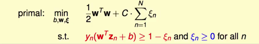
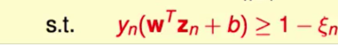
这个是soft-margin SVM的原问题:
我们知道用核技巧,其实就是把$x$映射到$z$空间上,而$pK(x,x’)+q$这样的改变中,$q$平移空间是不会影响结果的,而$p$拉伸空间是可以改变结果的,所以我们只考虑$p$即可。
$K$变成原来的$p$倍,那么$z$就是原来的$\sqrt{p}$倍,这样我们为了这个不变化:
$w$就要变成原来的$\frac{1}{\sqrt{p}}$倍,那么为了使下式子不被影响到:
由于$\frac{1}{2}w^Tw$变为了原来的$\frac{1}{p}$倍,那么C也要变为原来的$\frac{1}{p}$倍。
即答案为第五个。
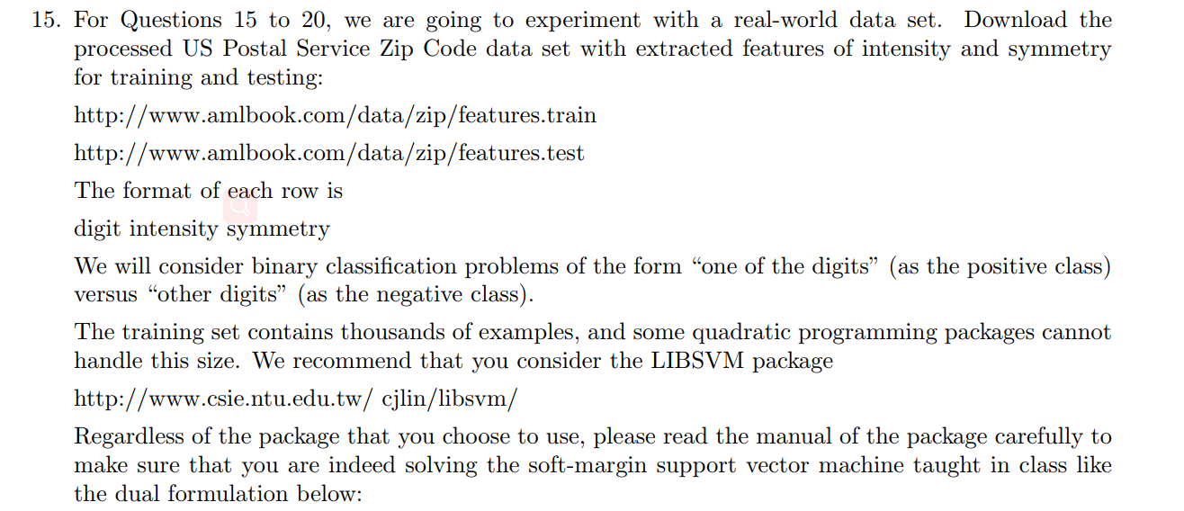
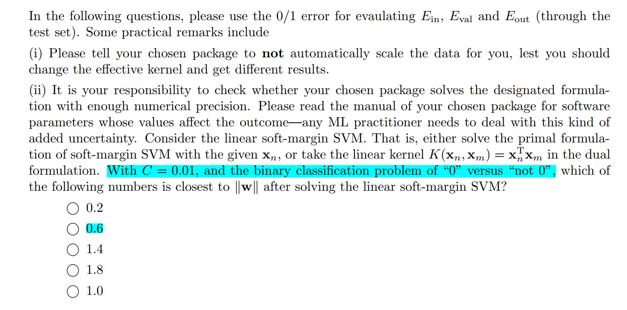
Q15
1 2 3 4 5 6 7 8 9 10 11 12 13 14 15 16 17 18 19 20 21 22 23 24 25 26 27 28 29 30 31 32 33 34 35 36 37 38 from cvxopt import solvers, matriximport numpy as npimport matplotlib.pyplot as pltimport sklearn.svm as svmimport mathdef splitData (path) :for line in txt:0 ])))1 ]), float(linesplit[2 ])])return np.array(data_x), np.array(data_y)def classificationFunction (dataOfy, target) :for _ in dataOfy:if _ == target:1 )else :0 )return np.array(newdata_y)if __name__ == '__main__' :"train.dat" )0 )0.01 , kernel='linear' )
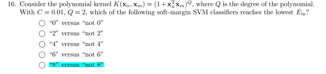
Q16
1 2 3 4 5 6 7 8 9 10 11 12 13 14 15 16 17 18 19 20 21 22 23 24 25 26 27 28 29 30 31 32 33 34 35 36 37 38 39 40 41 42 43 44 45 from cvxopt import solvers, matriximport numpy as npimport matplotlib.pyplot as pltimport sklearn.svm as svmimport mathdef splitData (path) :for line in txt:0 ])))1 ]), float(linesplit[2 ])])return np.array(data_x), np.array(data_y)def classificationFunction (dataOfy, target) :for _ in dataOfy:if _ == target:1 )else :0 )return np.array(newdata_y)if __name__ == '__main__' :1 0 for i in range(9 ):"test.dat" )"train.dat" )0.01 , kernel='poly' , degree=2 , gamma='auto' )if 1 - correct_num/test_data_y.shape[0 ] < Ein:1 - correct_num/test_data_y.shape[0 ]
Q17
1 2 3 4 5 6 7 8 9 10 11 12 13 14 15 16 17 18 19 20 21 22 23 24 25 26 27 28 29 30 31 32 33 34 35 36 37 38 39 40 41 42 43 44 45 46 47 48 from cvxopt import solvers, matriximport numpy as npimport matplotlib.pyplot as pltimport sklearn.svm as svmimport mathdef splitData (path) :for line in txt:0 ])))1 ]), float(linesplit[2 ])])return np.array(data_x), np.array(data_y)def classificationFunction (dataOfy, target) :for _ in dataOfy:if _ == target:1 )else :0 )return np.array(newdata_y)if __name__ == '__main__' :1 0 0 for i in range(0 , 9 , 2 ):"test.dat" )"train.dat" )0.01 , kernel='poly' , degree=2 , gamma='auto' )if 1 - correct_num/test_data_y.shape[0 ] < Ein:1 - correct_num/test_data_y.shape[0 ]if np.sum(np.fabs(clf.dual_coef_)) > maxxalpha:
Q18
Q19
1 2 3 4 5 6 7 8 9 10 11 12 13 14 15 16 17 18 19 20 21 22 23 24 25 26 27 28 29 30 31 32 33 34 35 36 37 38 39 40 41 42 43 44 45 46 47 from cvxopt import solvers, matriximport numpy as npimport matplotlib.pyplot as pltimport sklearn.svm as svmimport mathdef splitData (path) :for line in txt:0 ])))1 ]), float(linesplit[2 ])])return np.array(data_x), np.array(data_y)def classificationFunction (dataOfy, target) :for _ in dataOfy:if _ == target:1 )else :0 )return np.array(newdata_y)if __name__ == '__main__' :1 0 0 for gamma in [1 , 10 , 100 , 1000 , 10000 ]:"test.dat" )"train.dat" )0 )0 )0.1 , kernel='rbf' , gamma=gamma)if 1 - correct_num/test_data_y.shape[0 ] < Eout:1 - correct_num/test_data_y.shape[0 ]
Q20
1 2 3 4 5 6 7 8 9 10 11 12 13 14 15 16 17 18 19 20 21 22 23 24 25 26 27 28 29 30 31 32 33 34 35 36 37 38 39 40 41 42 43 44 45 46 47 48 49 50 51 52 53 54 55 from cvxopt import solvers, matriximport numpy as npimport matplotlib.pyplot as pltimport sklearn.svm as svmimport mathimport randomdef splitData (path) :for line in txt:0 ])), float(linesplit[1 ]), float(linesplit[2 ])])for line in data:0 ])))1 ]), float(linesplit[2 ])])return np.array(data_x), np.array(data_y)def classificationFunction (dataOfy, target) :for _ in dataOfy:if _ == target:1 )else :0 )return np.array(newdata_y)if __name__ == '__main__' :1 : 0 , 10 : 0 , 100 : 0 , 1000 : 0 , 10000 : 0 }for _ in range(100 ):1 0 for gamma in [1 , 10 , 100 , 1000 , 10000 ]:"train.dat" )0 )0.1 , kernel='rbf' , gamma=gamma)0 :1000 ], train_data_y[0 :1000 ])0 :1000 ])0 :1000 ])if 1 - correct_num/1000 < Eout:1 - correct_num/1000 1